DESeq2 normalization
With the RNA-seq read count data (that hasn't been transformed, normalized, etc), you're ready to use the
DESeq2 pipeline to produce an analysis of your data. There is a lot that happens under the hood in DESeq2
and we'll go into some level of detail.
One important part of the DESeq2 pipeline is normalization of your raw read counts. Normalization in general
refers to when data is transformed in a way to reduce the impact of a confounding variable that could skew
the results of an analysis.
The normalization of RNA-seq data is well-explained by this
StatQuest video, but I'll summarize the major points here. The two confounding factors that DESeq2 normalization
accounts for is sequence library size and composition.
Library size refers to the total number of reads in one sample. Hypothetically, if sample 1 has a total of 100 reads
across 3 genes, whereas sample 2 has a total of 500 reads for the same 3 genes, we might conclude that sample 2 has a
much higher expression of each of the three genes relative to sample 1, when in fact, that isn't the case.
Library composition refers to when two samples have certain genes that have very different expression levels as a
biological property as opposed to because of the experiment conditions. For example, intestinal epithelium might express
a gene at a high level whereas liver cells don't epress that gene at all. If the library size is the same for both samples,
the expression of that particular gene in intestinal epithelium might affect the observed expression of other genes in
intestinal cells, which makes it difficult to compare with liver cells.
The mathematics behind DESeq2 normalization is not extremely complex, but is more detail than we need right now. Essentially,
a scale factor is calculated for each sample to control for the effects of library size and composition. How the scale factor
is calculated is described in detail in the StatQuest video. If you're interested in what the algorithm looks like in R, the
code is shown below.
            logData <- log(data)
            geneAvgs <- rowMeans(logData)

            logData <- logData[geneAvgs>0, ]

            geneAvgs <- geneAvgs[geneAvgs>0]

            logRatios <- logData-geneAvgs

            sampleMedians <- apply(logRatios, 2, median)

            sampleScalingFactors <- exp(1)**sampleMedians

            normalizedData <- sweep(data, 2, sampleScalingFactors, `/`)
            head(normalizedData)
We'll see in a minute that the code above is really unnecessary if we want to access the matrix of normalized
counts after DESeq2 processing.
Running DESeq2 on a data set
To actually run DESeq2 on a dataset, we first make a DESeqDataSet object with the parameters of our experiment with the DESeqDataSetFromMatrix function. Here, we specify the matrix containing our read counts, the sample description, and the design parameter. The design parameter allows you to inform DESeq2 of the scheme of your experiment. For example, for our use, we just specify ~exp.control so that DESeq2 knows we want to compare expression levels between samples with different values for the exp.control column. In this case, this would be comparing WT vs KO samples. More complex designs are possible and we'll describe how they work later.
            library(DESeq2)
            dds = DESeqDataSetFromMatrix(countData = data, colData = sample_desc, design = ~exp.control)
            dds = DESeq(dds)

            keep10 = rowSums(counts(dds)) >= 10
            dds = dds[keep10, ]
            dds
FYI, dds is a common name for your DESeqDataSet objects. Also, you'll notice that we filter the dds for rows (genes)
that contain less than 10 counts total across all columns (samples). 10 is a roughly arbitrary number, but the idea is that
if a gene has less than 10 counts across all samples, it likely isn't relevant for comparison.
A quick revisit to normalization again, to access the DESEq2 normalized counts matrix, all we need to do is run our raw
count matrix through DESEq2 and then use counts(dds, normalized = TRUE). As a general lesson, anything you can think of in
the course of your work has probably been thought of before and already exists, so it saves a lot of time to search for the
functionality instead of reinventing the wheel as we did above showing the algorithm of DESEq2 normalization in R.
To see the effect of DESeq2 normalization, we can use a bar graph showing the library size of each sample before and after
normalization.
            par(mar=c(8, 4, 4, 1) + 0.1)
            barplot(colSums(data)/1e6, las = 3, main = "Raw read counts per sample", ylab = "Millions of reads")

            normalized_counts <- counts(dds, normalized=TRUE)

            par(mar=c(8, 4, 4, 1) + 0.1)
            barplot(colSums(normalized_counts)/1e6, las = 3, main = "Normalized read counts per sample", ylab = "Millions of reads")
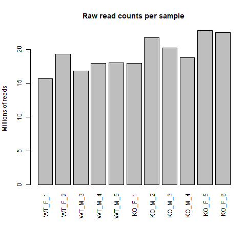
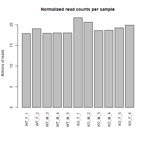
Just by eye, we can see that the distribution of library size for raw read counts is much more varied compared to after normalization. In the normalized read counts bar chart, we see that sample KO_F_1 and KO_M_2 are potential outliers in terms of library size so it is up to us if we want to exclude those samples and re-run DESeq2. I will not for this tutorial, but it is a valid concern as RNA-seq experiment can be sensitive to how they were conducted and potentially skew the results if outliers are not addressed.